Algorithmic Beauty: An Introduction to Cellular Automata

An overview of simple algorithms that generate complex, life-like results.

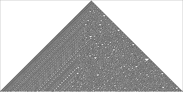The famous rule 30; capable of generating pseudo-random numbers from simple/deterministic rules. Rule 30 was discovered by Stephan Wolfram in ’83.

If you’re interested in the philosophical implications of cellular automata, check out my post here.

Cellular Automata (CA) are simultaneously one of the simplest and most fascinating ideas I’ve ever encountered. In this post I’ll go over some famous CAs and their properties, focusing on the “elementary” cellular automata, and the famous “Game of Life”. You won’t need to know coding to read this post, but for more technical readers I provide endnotes and Github repos.

I’ve also written a library in Python to generate the CAs which I use throughout the post. I didn’t like many of the ones I was encountering elsewhere on the internet because I felt they weren’t beginner friendly enough [1]. All the code is on Github, so you can read through it:

• Link to elementary CA library

• Link to Game of Life library

Cellular Automata Basics: The Elementary CAs

CAs are computational models that are typically represented by a grid with values (cells). A cell is a particular location on a grid with a value, like a cell on a spreadsheet you’d see in Microsoft Excel. Each cell in the grid evolves based on its neighbors and some rule.

Elementary CAs are visualized by drawing a row of cells, then evolving that row according to a rule, and displaying the evolved row below its predecessor. All this being said, they’re easiest to understand by example:

Rule / Key:

***  **-  *-*  *--  -*-  --*  ---  -**
 -    -    -    *    *    *    -    * 

$ python3 Main.py --evolutions 8 --rule 30
                            -------*--------
                            ------***-------
                            -----**--*------
                            ----**-****-----
                            ---**--*---*----
                            --**-****-***---
                            -**--*----*--*--
                            **-****--******-              

The above is an example of a CA. Here’s how it was generated:

• First, we start at the top row of cells. The top row of cells is a hand-chosen initial configuration. The values of the top row could be anything: they could be random, or just have 1 star in the middle, as we have here. The CA will do drastically different things based on the initial conditions, but typically the same sorts of shapes will appear.

• Each cell from the 2nd row onwards is computed based on its own shape and the shape of its neighbors above according to the key on the top. Cutoffs are counted as “-”s. For example, row 2 column 2 is a “-” because there is a “-” “-” “-” above it, as described in the 2nd to last rule of the “Rule” above. Note that all the cells in the row evolve in parallel.

The elementary CAs are often referred to as “rules” (reason why at [2]). The above CA is rule 30. Remarkably, it turns into the pattern at the top of the page if you run it for enough iterations. What’s more perplexing to experts is that despite the simple, deterministic, rules used to build the automata up, the results never converge. In other words, rule 30 never begins to exhibit any pattern in its behavior that would allow someone to predict what cells were in what state at an arbitrary row without computing all the iterations prior by brute-force. Throw any statistical tool you want at it, you won’t find anything of interest. This is interesting because most other patterns like it can be expressed algebraically, so when scientists want to know what will happen in a particular row, they can do some quick math and find out almost instantly. However, with rule 30, if we wanted to figure out what happens on the billionth row, we would actually have to generate all 1 billion rows, one by one! For this reason, rule 30 actually served as the random number generator in Mathematica for a long time.

This pseudo-random behavior is what makes rule 30 so fascinating. How could something built from deterministic rules be both so beautifully ordered and impossible to predict? We’ll see this behavior in CAs that move “in time” as well; these exhibit almost lifelike behavior.

Most CAs don’t have this random behavior; they converge to well-defined patterns. Take rule 94:

Rule 94. Source .

Another CA that can produce random behavior is Rule 90. There are a lot of special things about rule 90; one of them is that is can behave predictably, or randomly based on its initial conditions. Check it out.

Rule/key
*** **-  *-* *-- -** -*- --* ---
 -   *    -   *   *   -   *   - 

python3 Main.py --evolutions 8 --rule 90
                      -------*--------
                      ------*-*-------
                      -----*---*------
                      ----*-*-*-*-----
                      ---*-------*----
                      --*-*-----*-*---
                      -*---*---*---*--
                      *-*-*-*-*-*-*-*-

Notice how in the above diagram a single star in the middle produces highly self-similar behavior. Here’s an expanded of the same pattern. You’ll probably recognize this Sierpiński triangle fractal.

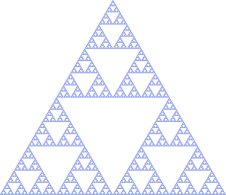
In this configuration rule 90 is predictable. But let’s see what happens when we give it a random initial configuration instead:

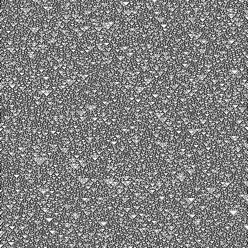Rule 90 again. Same rule as above, but with a random initial condition. This time the individual cells are unpredictable, like in rule 30.

This is what mathematicians and philosophers mean by *sensitivity to initial conditions. *Most of the functions you’ve studied in school don’t behave this way.

These three should give you a good idea of what elementary CAs are like. They’re only called elementary because each cell only has two states: colored, and not colored (I use * and “-” for colored and not colored, but in principle, this is the same).

CAs were originally discovered by John Von Neumann and Stanislav Ulam in the 40s, but many of the CAs I talk about here weren’t found until modern computers allowed researchers to explore the space of potential CAs quickly. More contemporarily, Stephan Wolfram, the founder of Wolfram Alpha, has studied the elementary CAs exhaustively [3]. He’s shown that random patterns like the one exhibited in rule 30 don’t become any more likely when the CAs are no longer elementary. If you’re looking for more resources on elementary CAs, his book, *A New Kind of Science, *is probably the best resource I’ve found.

Now that you know what elementary CAs are, you’ll start noticing them everywhere. Pretty amazing for such a recent discovery.

Shellular automata. Source

2D Cellular Automata: Conway’s Game of Life

Now that you’re familiar with the basic “1D” CAs, I want to show you what you can do with 2D CAs. The results are remarkable because the CAs look to be “alive”. Whenever I run these programs I feel like I have a petri dish living inside my computer.

This is what I mean when I say the results look like they’re out of a petri dish.

The 2D CA I want to show you is called “Conway’s Game of Life”, or just Life, *as it’s referred to often in the literature. Its name and appearance are not an accident. The creator of *Life, John Horton Conway, built it with the intention that it satisfied John von Neumann’s two criteria for life.

(As I mention in the introduction, I wrote a library to run the game of life in the terminal that you can use to play around with these quickly if you have basic programming expertise.)

Von Neumann viewed something as being ‘alive’ if it could do two things:

1. Reproduce itself

2. Simulate a Turing machine

Conway succeeded in finding a CA that fit these criteria. The “creatures” in the game seem to reproduce, and, after some efforts, researchers have proven that Life is, in fact, a universal Turing machine. In other words, Life can compute anything that is possibly computable, satisfying item 2 [4].

As we saw with the elementary CAs, the rules of Life are simple to implement. But instead of considering neighbors in the row above the cell-like we did with the elementary CAs, Life counts the neighbors surrounding a cell to decide the state of the cell in the middle. Unlike elementary CAs, the next generation of cells is displayed as a “game tick” instead of another row of cells beneath the previous. Here are the rules:

1. Any live cell with fewer than two live neighbors dies, as if by underpopulation.

2. Any live cell with two or three live neighbors lives on to the next generation.

3. Any live cell with more than three live neighbors dies, as if by overpopulation.

4. Any dead cell with exactly three live neighbors becomes a live cell, as if by reproduction.

It’s worth noting that typically the grid that the cells live on will have a toroidal geometry — think pac-man style —where cells will “loop around” to look for neighbors.

Amazingly, the above rules generate the complex patterns above. Here’s another example of Life, this time earlier in its evolution, and made using the Github repo I mentioned earlier:

Short gif of the output of the Github repo I wrote. Notice how some collisions seem to spawn multiple “creatures” while others leave some live cells in stasis. When given a large enough grid, this configuration will actually expand indefinitely instead of “going extinct” as many others do.

We aren’t limited to random-looking shapes though. There are a number of patterns, or “attractor states” that Life tends towards. Below is a collision between two of them. I love how the rules above can generate a sort of collision detection by themselves.

A collision between a pulsar (the big, oscillating structure) and a glider (the smaller thing, traversing the map). Without a collision, both will continue on indefinitely.

These are just a few of the properties of Life. If you’re interested, definitely play around with the library I provide and read more. Also, keep in mind that Life is also far from the only 2D CA out there. If you want to check another out another 2D CA, I’d recommend Brian’s Brain.

I want to leave you with a video of some of the most astounding configurations of Life. I hope it leaves you with the same feeling of mystery it left me with.

Notes

**[1] **Much of the audience for CAs are philosophers, biologists, and high schoolers with only basic coding backgrounds. Most of the libraries I found had dependencies that could be complex for a beginner to install. I’d rather have something that people can run in the shell and see what’s going on immediately.

[2] What is this numbering system? (The Wolfram Code)

Wolfram also invented the numerical code that we’re using to name each rule. The numbering system requires you to understand binary, so feel free to skip this section if you don’t know binary. The number of the given rule tells you how it should react to different inputs. Here’s an example: rule 90 is 01011010 in binary. The ith digit of the binary encoding tells you how the rule behaves for input i. So rule 90 outputs a 0 for input 111 because its digit in the 8th’s place is 0 when converted to binary. Note that *** is 111 in the diagram below, which is 8 in decimal.

This is easier to see visually:

Visualization of how we come to the names “rule 90” and “rule 30”.

**[3] **Admittedly, I haven’t finished his 1,200-page book *“A New Kind of Science”. *It’s sitting in my apartment, looking at me kind of eerily. Most of it is pictures, so I’m about 200 pages through though. I’d probably finish it if it wasn’t so heavy.

**[4] **I know this is a big statement to gloss over in a single sentence. I may do another post on Turing machines and their relationship to CAs and philosophy in another post.