Machine Learning ISIC Cancer Classification Challenge 2 Deep Learning with AWS

This is a tutorial on building and a basic transfer learning model for the ISIC challenge. It’s a sequel to my first ISIC challenge post which you can find here, but can be read independently as well.

It’s well known that the state of the art the last few years for image classification has been dominated by convolutional neural network (CNN) techniques trained on massive data sets numbering in the millions. However, in the medical imaging domain datasets remain comparatively small. In melanoma classification most datasets number in the thousands of samples, some papers try to make due with even fewer, but classifiers trained on such small dataset rarely generalize well. Successful melanoma classification systems like this one published in Nature have employed transfer learning to help overcome limited training sizes.

Transfer learning works by taking some of the parameters learned on a large dataset and utilizing them on a smaller dataset. In image recognition this involves “freezing” the parameters for some number of convolutional layers from a pre-trained CNN to use as a feature extractor, then re-training the final fully connected layers of the network for a new problem in hopes that the feature extraction learned on the previous dataset will prove useful for the new one.

In this post I won’t focus much on the theory behind CNNs and transfer learning, but I can recommend some resources if you’re unfamiliar with them. Instead, I want to focus on theprocessof building and improving a transfer learning model. First we’ll discuss the ISIC challenge itself and the role the cloud can play in building classifiers. Then we’ll retrain a typical transfer learning model on AWS and analyze it. Towards the end we’ll also lightly go over some techniques like stacking that can give you top-notch performance.

Later in the post I’ll link to all of the associated code, so you should be able to duplicate the work in a few minutes of dev-time provided you have an AWS account already.

For our dataset we’ll look to the ISIC melanoma classification challenge.

If you’re interested in some more background on the ISIC challenge, newer to machine learning, or you just want to see what a basic classification system for that challenge would look like with no mention of infrastructure, check out my previous post where I build a basic principal components analysis + decision tree based model for the 2017 challenge.

To follow the steps in this post I’m only assuming that you’ve created an AWS account, you’veinstalled the AWS CLI, and exported the credentials locally as environment variables. You don’t even need to have Tensorflow installed locally! Some basic AWS knowledge is useful here (e.g. what are EC2 and CloudFormation), but not required.

The Dataset

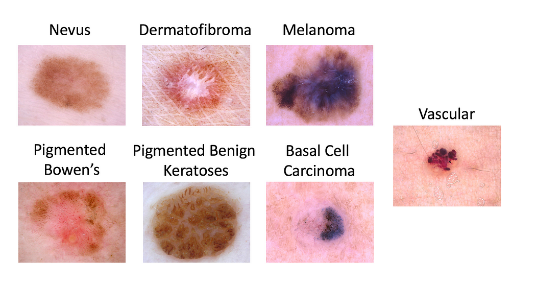
The ISIC has just released their 2018 challenge. This year the classification challenge changed from focusing on whether or not to biopsy (binary classification) to a full multi-class classification problem including 7 different types of lesions.

The desired metric for the ISIC challenge this year is 7-way classification accuracy, not AUC as it has been in previous years. However, to keep the results consistent with my previous post, I’ll still only going over benign vs. malignant classification in this post. Changing the results to get the 7-way accuracy merely requires changing the directory structure I’ll describe later in the post. Submissions still require presenting an AUC value for melanoma vs. rest, but it is no longer the target metric.

Why Train in the Cloud?

Before we jump into the code here are a few things motivating this approach (in no particular order):

1. The transfer learning script we’ll use in this post freezes all of the convolutional layers of the CNN, so it can be accomplished on a normal CPU. However, fine-tuning some of the convolutional layers of the CNNs is often the optimal approach on datasets this size, and that warrants the use of a high end GPU due to the increase in the number of parameters you need to train. In the approach you’ll see below, using a GPU enabled instance is as easy as swapping out theInstanceTypein the template to use a P2 instanceinstead of at2.mediuminstance.Keep in mind that P2 instances are expensive! You’ll need to be careful to shut them down when you’re done using them.
2. If you need to train an ensemble of models, or have multiple experiments you need to run in parallel (for K-folds), spinning up an instance for each experiment is as easy as rerunning the small number of commands in the below section, but for a CloudFormation stack with a different name. Giving each stack a different name will also let you manage your experiments and their associated infrastructure easily.
3. Using an AMI with all of the major deep learningframeworks pre-installed will save us a lot of time that could have been wasted on configuration. When different experiments call for different libraries or frameworks we’ll be able to use the same code to stand up any experiment independently of all others.
4. If you’re like me, and you don’t want to leave your computer on for hours, this approach will let you start training the model and walk away.
5. Using a CloudFormationtemplate will let us version control our infrastructure, and turn spinning the instance up into a single command. It will also make getting the IP of the instance even easier. If we wanted something like a S3 bucket to store our models that would also belong here.

The Infrastructure

For this post we’re going to train our model on an AWS EC2 instance using an AMI. We’ll also template out all of our code in AWS CloudFormation.

Before you execute the code below please remember that because you’re spinning up real hardware it will charge your AWS account money.

---
AWSTemplateFormatVersion: '2010-09-09'
Description: Attach IAM Role to an EC2
Parameters:
  KeyName:
    Description: EC2 Instance SSH Key
    Type: AWS::EC2::KeyPair::KeyName
  InstanceType:
    Description: EC2 instance specs configuration
    Type: String
    Default: t2.medium
Resources:
  Learner:
    Type: AWS::EC2::Instance
    Properties:
      BlockDeviceMappings:
      - DeviceName: "/dev/sda1"
        Ebs:
          VolumeSize: '100'
      InstanceType:
        Ref: InstanceType
      ImageId: ami-d2c759aa
      KeyName:
        Ref: KeyName
      SecurityGroupIds:
      - Ref: SSHAccessSG
      Tags:
      - Key: Name
        Value: StackExample
  SSHAccessSG:
    Type: AWS::EC2::SecurityGroup
    Properties:
      GroupDescription: Allow SSH access from anywhere
      SecurityGroupIngress:
      - FromPort: '22'
        ToPort: '22'
        IpProtocol: tcp
        CidrIp: 0.0.0.0/0
      Tags:
      - Key: Name
        Value: SSHAccessSG
Outputs:
  EC2:
    Description: EC2 IP address
    Value:
      Fn::Join:
      - ''
      - - ssh ubuntu@
        - Fn::GetAtt:
          - Learner
          - PublicIp
        - " -i "
        - Ref: KeyName
        - ".pem"

The CloudFormation template we’ll use to start our EC2 instance. Including a CloudFormation mapping for the different AMIImageIds in each region is a best practice I left out of the above template for brevity.

The only issue I’ve found with this approach is that theImageIdparameter can be difficult to track down. If you’re having issues finding a specific Image ID for another region, let me know and I can help you (it’s actually a surprisingly tricky process). TheImageIdis also updated regularly, so if this one out of date please let me know.

Here’s how to set up this template (assuming your AWS credentials are stored as environment variables, and you have the AWS CLI installed):

I’m going to assume you’ve got JQ installed. It will let us parse JSON in our shell much more easily, and the install is pretty simple. First install the above template locally, then follow these commands:

# Create a key pair we'll use for securely ssh'ing into our instance
aws ec2 create-key-pair — key-name Key | jq -r ‘.KeyMaterial’ > Key.pem

# Create the EC2 instance we'll train our model on (this is called a "stack" in CloudFormation)
# We'll use the above cloudformation template and assuming it's called basic-template.yml locally and in your
# working directory
aws --region us-west-2 cloudformation create-stack --stack-name Learner \
  --template-body file://basic-template.yml \
  --parameters ParameterKey=KeyName,ParameterValue=Key --capabilities CAPABILITY_IAM
  
# Wait a little bit for your virtual machine to start... (usually just a few minutes)

# Get your SSH command to log into the EC2 box
aws --region us-west-2 cloudformation describe-stacks --stack-name Learner | jq -r '.Stacks[0].Outputs[0].OutputValue'

# Example output: ssh ubuntu@34.216.115.46 -i MyKeyPair.pem

# ssh in to be sure everything is working 
ssh ubuntu@34.216.115.46 -i Key.pem

Downloading the Data

My process for downloading data included browsing the ISIC image galleryto understand the it, downloading the metadata for the dataset using the “download metadata” option on the gallery (I filtered the “SONIC” dataset using the gallery for reasons you’ll see below), then running a few of my own scripts to download the image data and put it into a suitable format.

I’ve put together a small repository on Githubcontaining the scripts I used to download the dataset. I prefer this approach because I’m using an EC2 box to run my classifier, and I don’t have much use for anything other than the testing data locally. The alternative would be to download the images from their ISIC website andscpthem to your EC2 box, but this would take much longer (and wouldn’t take advantage of multiprocessing).

# from your EC2 box
# start a tmux instance so we don't have to leave the terminal open while downloading
tmux 
git clone https://github.com/evankozliner/image-downloader.git
cd image-downloader
make
# Output:
# https://isic-archive.com/api/v1/image/558d6423bae47801cf735194/download
# https://isic-archive.com/api/v1/image/5436e3c2bae478396759f1f5/download
# https://isic-archive.com/api/v1/image/558d6165bae47801cf73487f/download
# ...

# ctrl+b+d to exit tmux and leave the images downloading

One “Gotcha” in this dataset

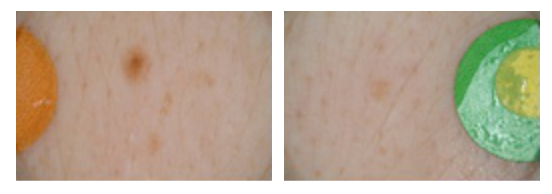
If you download the images through the API I describe above, you may want to consider filtering the metadata from the “SONIC” dataset. SONIC is a 9000 image large dataset containing entirely benign moles in children. Not only will including the SONIC sample heavily bias your benign lesions towards moles, but all of the images I could see in the dataset appear to include this large colored circle that the classifier will learn to diagnose as being benign. The first time I ran this classifier I accidentally included this dataset and got some suspiciously high accuracies in the mid 90s under a 60/40 benign/malignant split, so don’t make my mistake.

Training a Classifier

When I was originally writing this tutorial I considered adding a more complex model to it, but there are already many excellent tutorials on doing that, so I want to focus on bringing up the infrastructure here. Now that you have an AMI available with all of the popular deep learning libraries pre-installed on it you’re open to any kind of experiment you’d like to do, so any other tutorials you find on neural networks should work on this instance (I link to some in “Next Steps”).

For the remainder of this tutorial I’ll show you how a quick transfer learning model performs. There’s animage retraining samplethatTensorflow provides a tutorial onthat is perfect for seeing basic transfer learning results quickly, but if you want to include the transfer learning model in an ensemble, do fine tuning on your network, or any analysis beyond seeing your accuracy you’ll need to modify it slightly, or if you don’t know Tensorflow well enough consider another solution like Keras.

If you’d like to have some more fine-grained analysis of the model, I have aTensorflow fork on Githubwhere I add the logging necessary to generate the ROC curve I show in “Analyzing our Results”. Forking the whole Tensorflow repo wasn’t totally necessary here, but it does help emphasize that the script was not my work.

# From the EC2 box you've ssh'd into 
# start tmux so we don't need to stay on the instance while it trains
tmux attach
cd ~
# this will install a tensorflow version optimized for your instance (CPU or GPU)
source activate tensorflow_p36
# assuming you've used the image downloading script mentioned above to put your images in the ~/images directory 
# consider adding more tags for data augmentation like --random_crop 5 or --flip_left_right 
python src/serving_tensorflow_p27/tensorflow/tensorflow/examples/image_retraining/retrain.py --image_dir ~/images

# while it's training hit ctrl+b+d to exit tmux but leave the training going 

Analyzing Your Results

ROC curves are an excellent way to measure our performance in a 2-class classification problem where the dataset is imbalanced. Oftentimes we’ll also be interested in how our model performs when artificially increasing its false-positive rate. In the ISIC challenge we’re interested in a low false-positive rate because it equates to a low rate of unnecessary biopsies. I go a little more in-depth into the ROC curve inmy previous post on the ISIC challenge, but for those who are unfamiliar the ROC is a plot of the true-positive-rate and false-positive-rate at different classification thresholds; it’s built by picking classification thresholds and re-computing the true-positive-rate and false-positive-rate the model would achieve on the test set. ROCs are often judged by their area under the curve (AUC).

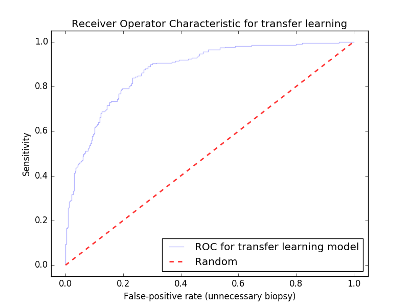
It’s not totally fair to compare this model with the previous posts’ because it was trained with a larger data set, but even without any data augmentation, ensembles, or fine-tuning we’ve outperformed our previous model by .06 AUC, and this model was far easier to build. There’s still a chance that this model did not perform better than the PCA to decision tree model discussed in my last post though, so in practice it would be wise to perform some cross-validation on it. Because the model takes some time to train, cross validation is another place where running several AWS instances in parallel can come in handy (you’ll need to train the the classifier on each instance with a different set of training / testing data to accomplish cross validation here).

Improving Your Classifier

A .86 AUC isn’t bad, but it’s hardly world-class, top papers tend to be in the mid 90s. The easiest solution to increase our AUC here would be to get more images, but in light of that I thought it could be good to discuss some next steps to try and squeeze a bit more out of the classifier. I talk about some of these a little in my previous post as well, and any of the techniques I mention there will also help improve CNN’s score.

Fine tuning

Fine tuning is the process of retraining more than just the final fully connected layers of a neural network while transfer learning. In image classification this will usually involve additionally re-training the convolutional layers in addition to the final fully connected layers. It’s especially useful for image classification problems like the ISIC because the later convolutional layers of the CNN tend to apply more dataset-specific feature extractions, which are less likely to be useful for us if they’ve come from datasets like ImageNet.

If you’re interested in fine tuning a model, it might be best to move away from the script I use in this post and utilize a high level library like Kerasfirst. In Keras the process of un-freezing and fine tuning some of the later convolutional layers is simpler than in frameworks like Tensorflow. You could still utilize the AWS AMI the way I describe it above, but as I mentioned previously it would be best to train the model on something like a P2 instance while fine tuning because upon un-freezing some layers of the network the training will be significantly slower without a GPU.

Here’s an excellent tutorial series on how to accomplish this in Keras.

Preprocessing

Outside of standard techniques like normalization, image segmentation is probably the most useful preprocessing technique commonly applied to melanoma classification. Segmenting the image improves AUC by removing noise that might otherwise fool the classifier.

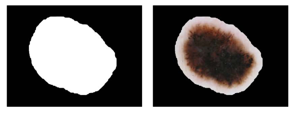
In segmentation a “mask” (left) is found for the image, and the coordinates of the mask are used to “crop” the image (right). Reference:Jack Burdick, et all. This helps the classifier by removing background noise on the image.

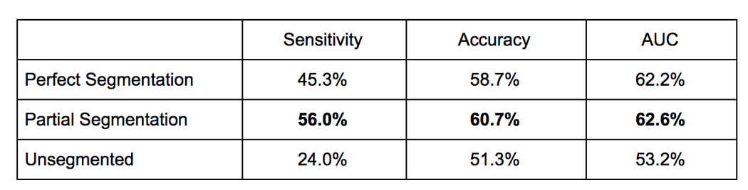
Above is an empirical experiment out of Florida Atlantic University that suggests that partial segmentation is ideal for CNN models. Reference:Jack Burdick, et all

Segmentation is a separate challenge in and of itself, and it’s another case where various convolutional architectures have proven to be the state of the art. Traditional image segmentation approaches like thresholding are still useful here, but in my experience they run into trouble when encountering common “distractions” like hair.

Ensembles

Using an ensemble of learners is another popular approach. Ensemble learners run new examples through multiple classifiers and then combine the results, usually through some kind of weighted voting. You’ll need to train (and cross-validate) each classifier in the ensemble separately, so this is where the ability to spin up arbitrary numbers of servers with something like AWS becomes incredibly valuable.

Your options for how to ensemble are wide; here are some successful ensembles I’ve seen:

• Traditional machine learning techniques trained with handcrafted features together with deep learning approaches like the one I described in this post.
• Ensembles of different deep learning architectures (say VGG16 and Inception V3).
• Ensembles where one classifier is trained on segmented images, and another is trained on the full image.
• Ensembles of separate binary classifiers combined using a linear approximation. For example using a sebhorratic keratosis vs. others classifier alongside a melanoma vs. others classifier.

Here’s a good tutorial on ensembles of convolutional networks.

Keep in mind that you’ll want your models’ results on the training set to be uncorrelated if you expect gain any information by combining them.

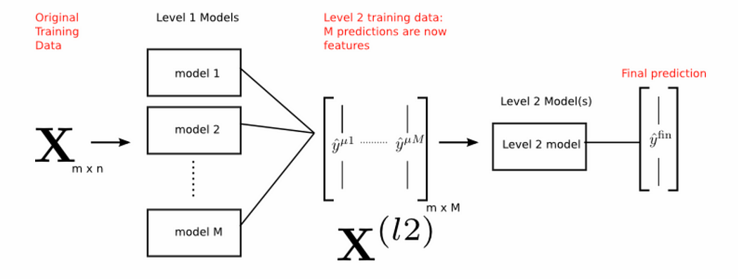
Another consideration is stacking models; this is essentially training another classifier on the outputs of your ensemble of trained classifiers. I haven’t seen very many papers abuse this technique for the ISIC yet, so that could be a promising area to look in to.

And of course there’s nobody saying you can’t fine tune, utilize segmented images, and ensemble ;)

Final Remarks

If you’ve made it this far, thanks for reading! I hope you have an idea of how you might train a basic deep learning classifier on AWS, and how you could improve it with some more advanced techniques.

Remember to delete the stack once you’re done using it or you will be billed for more time than you intended.

If you find any mistakes anywhere please let me know! I probably haven’t proof-read this as much as I should.

And if you’re experiment with the ISIC challenge yourself I’d love to hear about your results and what you’re trying. Contact me on Medium, on Twitter, or at evankozliner@gmail.com. I’m incredibly excited to see what the 2018 papers look like :)